In life, as in art, the beautiful moves in curves..
|
|
February 2024—MAJOR RE-WRITE ALERT I’ve done a MAJOR re-write of all the Bézier curve routines. Yes. Nah, they’re not backward or any other kind of compatible with what they used to be. I’m not sorry. Instead of three different sets of routines, the new routines are universal for curves, shapes (The GHOUL’s polygons) and 3D solids. It’s all 'much more better'.[1] Let’s dive in. |
Introduction
Bézier curves are a thing of beauty, quite intuitive—once you get used to them—and very convenient to work with. They are used extensively in vector graphics, font descriptions like PostScript and SVG, robotics and animation, and they even have an application in CSS. The GHOUL has Bézier routines for 3D curve generation, polygonal shapes, and mesh generation for polyhedra.
This page has a lot of information, and many concepts to become acquainted with; it’s a bit of a curve—see what I did there? With nearly 9000 words, this is not a 5 minute read, but I’m confident you’ll be happy you took the time to work your way through it when you’re building smooth, flowing organic shapes like this gear-shift knob in OpenSCAD.
|
|
You would probably have written this library making choices different to mine; we’re different people. This is not the only way to do these things. I’ts probably not the best way either, but it seemed a good way to me at the time, so I’m asking you to bear with me. I have had a lot of time to get used to this library, and it may seem strange or awkward to you at first, once again: bear with me, and if you see a better way, please let me know, I’d be happy to hear your thoughts. |
A Bézier primer
Some properties
-
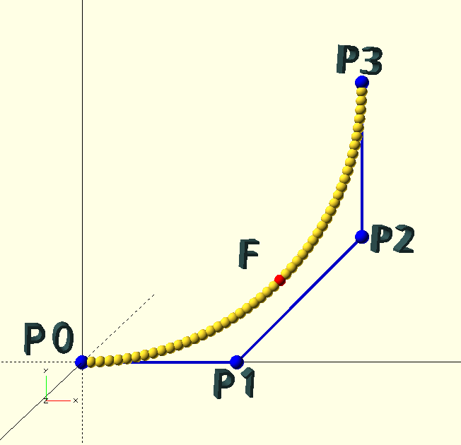
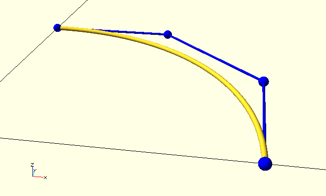
A Bézier curve is constructed from a set of 'control points' P0, P1 … Pn, of degree n, forming a 'control polygon'. A single point is—obviously—a point, two points give a straight line, three points (n=2, i.e., a 'quadratic' curve) or more can define effectively any curve. The curve in the image is a four point (n=3), or 'cubic' curve. Cubic curves are very convenient, as we will see, and The GHOUL’s routines are based on cubic Bézier curves, although you do have options.
-
The first and last control points, P0 and Pn are the endpoints of the curve, and are the only two points that are explicitly part of the curve. The remaining, intermediate, control points are not part of the curve, but influence it’s direction and curvature; imagine them connected to the curve with elastic bands, the greater their distance to the other points, the stronger their influence or 'pull'.[2]
-
The control polygon end-segments, i.e., P0 - P1 and Pn-1 - Pn are tangential to the the curve at their respective endpoints, i.e., the curve leaves an endpoint in the direction 'directly towards' the nearest control point.
-
There is no local control in Bézier curves; a change to any single control point affects the entire curve, although the effect diminishes with distance from the changed point. Only the two endpoints are fixed and do not move when any one of the control points changes. The GIF image in the Why cubic? section demonstrates this quite nicely, if I say so myself…
// A Bezier curve Control Polygon.

CP = [[0,0],[0.552,0],[1,0.448],[1,1]];
Mr. P. de Casteljau’s algorithm
Knowledge is power, and even though it’s all happening behind the scenes, it’s good to know how Paul de Casteljau’s algorithm works.
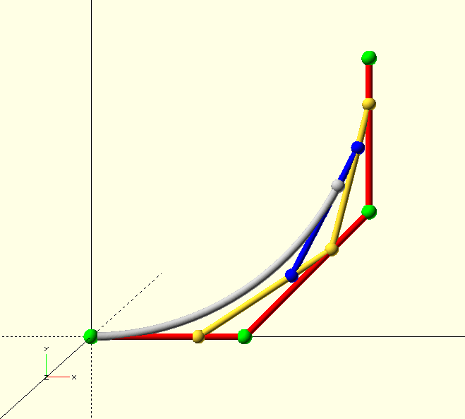
To find the 3/4 point of a cubic curve, the algorithm goes through the following steps.
-
Connect the control points (4 green spheres) with 3 lines (red).
-
Find the 3/4 point of each line (3 yellow spheres).
-
Connect these 3 points with 2 lines (yellow).
-
Find the 3/4 point of each line (2 blue spheres).
-
Connect these 2 points with 1 line (blue).
-
Find the 3/4 point of this line, (white) this is the point we seek.
Six interpolations are required for each point on the curve. If we want a curve with a resolution of 100 points, that’s 600 interpolations. Let’s just be glad we’re not doing this with a slide-rule.
Why cubic?
Because its Bernstein polynomial form is a 3rd order function, a Bézier curve with four control points is known as a 'cubic' Bézier curve, and it’s the most practical curve to work with; it has many applications, just check it out on Google, there is even a CSS implementation of it, and as we will see, with good reason.
The location of the endpoints of Bézier curves are always explicitly defined, but cubic Bézier curves are the lowest order Bézier curves that also define the tangent to the curve separately at each of the endpoints—since the end-sections of the control polygon form the tangents. Finally, the curvature or local 'radius' of the curve is—quite intuitively—determined by the distance between an endpoint and the adjacent control point. A larger distance will 'pull' the curve more in the direction of the control point before it turns away towards the other endpoint (see the animation here).
|
|
A cubic Bézier curve is the simplest Bézier curve that gives us control over the location, direction and curvature at each end of the curve individually. |
Having more than four control points—ironically—makes it much harder to control the curve; the effect of additional points is much less intuitive because each point influences the entire curve; it is better to split the curve into a number of cubic Bézier curves and maintain maximum control over the shape of the curve. After a little familiarisation, it’s easy to 'see' a cubic Bézier curve just by looking at the control points; with more control points, this becomes increasingly difficult, unless perhaps you have a brain that can win 10 games of chess at county level, simultaneously, blind.
For these reasons, The GHOUL’s routines use cubic Bézier curves, and I’m not dwelling on anything else here, however, BezierCurve() will let you work with Bézier curves of any order. If you must…
Smooth transitions
To create a smooth, continuous compound curve from multiple cubic curves, the following must be true:
-
The end- and start-point and their respective adjacent control points are collinear (all four points are on one line).
-
The end-point of the first curve coincides with the start-point of the next curve. If this is not the case, The GHOUL will put a straight section between the two, i.e., even though the curve will be continuous, the curvature will not be.
When both conditions are met, compound Bézier curves have a smooth, continuous transition between the partial curves.
|
|
Cubic Bézier curves can describe direction changes of around 90 degrees—whether circular or otherwise—quite accurately; direction changes of up to 180 degrees can be described somewhat satisfactorily, but beyond that, cubic Bézier curves are pretty useless. In general, if you want to keep adequate control, you must split your curves roughly at every 90 degrees of directional change. |
Circle approximation, and practical limits.
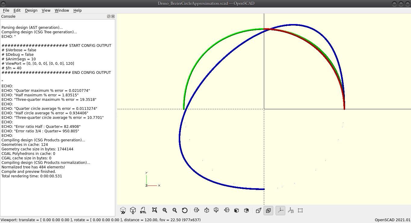
A cubic Bézier curve can approximate a quarter circle with only 0.021% maximum radial error—providing the right choice of control points. The closest approximation of a half circle with a single cubic Bézier curve is still—kind of—acceptable, it has a maximum radial error of 1.83%—more than 80 times worse. When we try to approximate a 3/4 circle with a single cubic Bézier curve, things really fall apart; just have a look at the image here, the maximum radial error is up to 19%, and the curve is more elliptical than circular—yes, that’s the closest you’ll get. Have a good look at the first quadrant in the image—click it; it opens in a new tab.
|
|
A single cubic Bézier curve is great at defining a curve through a 90° change of direction, pretty good up to 180°, and utterly useless after that. Break curves up into two or more partial curves whenever a directional change of more than 90° needs to be defined. |
Obviously, there are simpler, and better ways to get a circular path than using Bézier curves, like Arc(), but I’m trying to prove a point here—oh, wait, I did, in the call-out above…
// For a quarter circle of any radius R:
function CP_QC(R)=[[R,0],[R,0.552*R],[0.552*R,R],[0,R]];

// For a half circle of any radius R:
function CP_HC(R)=[[R,0],[R,1.33334*R],[-R,1.33334*R],[-R,0]];

// For a 3/4 circle... Nah. Not with a single cubic Bézier, you don't.
The GHOUL conventions for Bézier curves
The GHOUL gives the user two methods to define Bézier curves. Control Polygons, as you’ve seen above, are the basic method, and the only one DeCastejau() accepts. Then there are Tangent Points, my attempt at a more intuitive method to define Bézier curves; they are the go-to method for defining complex curves, shapes and solids, but control polygons are still useful as a 'quick and dirty' method to define simple curves and shapes.
The CP, CPS and CPA
-
Control Point a 2D or 3D vertex, by itself meaningless.
-
CP, Control Polygon, a tuple of Bézier curve control points that define a curve.
-
CPS, Control Polygon Set, an array of control polygons, describing a compound Bézier curve, i.e., a curve broken up into multiple curves (pretty much any curve with more than a 90 degree direction change needs to be a compound curve).
-
CPA, Control Polygon Array, an array of CPS, describing either a complex curve (made from a number of compound curves), or a shape where each of the CPS describes a path, like in OpenSCAD polygons.
The CP, or control polygon, is the 'low level' way to define a Bézier curve, and it works great for individual curves. The CPS is simply a set of control polygons, and The GHOUL interprets it as a 'compound' curve, i.e., it will (try to) daisy-chain the individual curves in set into one curve.
CP_10=[ // Single curve.
         // First quadrant of a circle of r=10.
        [10,0,0],[10,5.52,0],[5.52,10,0],[0,10,0]
    ]
;

CPS=[ // Compound curve.
        CP_10, // Quarter circle segment.
        ...     // Additional curve segments.
    ]
;
The CPA is an array of CPS. Even though behind the scenes in The GHOUL, it’s used every time you define a shape or 3D solid, it’s not something you’d usually work with yourself. A CPA defines what I call here a 'complex' curve, which is a curve composed of compound curves, i.e., a curve made of curves made of curves; yes, things are getting murky…
|
|
Although The GHOUL internally translates a TPA into a CPA to generate solids, manually defining a solid CPA would be a terrible job, so BezierSolid() insists on a diet of TPA only.
|
CPA=[   // Array of CPS. >> A complex curve.
        [   // Set of CP. >> A compound curve.
            [   // Bezier CP. >> A single curve.
                [x,y,z],[x,y,z],...,[x,y,z] // Usually 4 control points.
            ],
            ...
        ],
        ...
    ];
What a lot of hassle…
Control points, and polygons, are a bit of a hassle, and there’s a better way to define Bézier curves, at least I think so, and I hope that—after you get used to it—you’ll agree:
|
|
The GHOUL’s concept of a tangent point is my attempt to find an intuitive way to define a curve or a solid body with a few vertices and 'curvature indicators'. If you read my ramblings about them for the first time, they may not seem intuitive at all, so I’ll apologise beforehand, and do my very best to make clear what has emerged from the murky depths of my mind. |
The idea is to find 'optimal' places on the curve or solid you’re designing, and to define this 'optimal place' with one vertex (for its location), and some vectors that define the curvature of the object at that location, two for a curve (forward and reverse), or four for a solid (forward and reverse, 'up' and 'down').
So what are these 'optimal places' of which I speak? Just like when you give a person directions to your house, you don’t tell them "go straight, then keep going straight, go straight some more", you tell them "turn right at the candy store, left at the lights, then right at the green house and you’re there." Change of direction is what matters, and here, 'direction' means 'curvature'.
|
|
Tangent points should (must) be placed wherever the location and/or curvature of the object needs to be defined (more or less) accurately. |
Remember that I mentioned that a cubic Bézier curve is excellent at describing a quarter turn, pretty good at describing an s-bend or even a half turn, but crappy at anything like a three-quarter turn? This means that even a simple shape like a circle, needs to be made from multiple Bézier curves (four, actually, for a circle) and so, we’re usually looking at a 'compound' curve, consisting of multiple 'curve-sections', or even a 'complex' one, consisting of multiple compound curves.
Looking at such a compound curve, tangent points are placed at the end-points of the individual curve-sections, or more appropriately, they are simultaneously the end-point of a curve-section, and the start-point of the next section. The 'curvature vectors' essentially describe where the adjacent Bézier curve control point is situated, relative to the tangent point’s vertex. Thus, two tangent points describe the cubic Bézier curve between them, and—if there is a curve segment before or after—the end- or start-curvature of those segments.
3D solids have tangent points with four vectors, since not only a curve 'around' the solid must be described, but also the curvature 'up and down' the solid.
|
|
To some degree, this is where the Art of Engineering Design comes into the picture; you need to have the desired shape in mind, and, with your mind’s eye, see where the tangent points need to be to be the most effective. It requires an understanding of Bézier curves, and a one-ness with the design. It’s something that needs to be developed. Some are born with an innate ability and an affinity for three-dimensional visualisation, some are not. Much can be learned to compensate for lack of in-born ability. Anyone can do it, it’s just harder for some than others. We are not equal. I hope this all makes sense to you, and the ability to visualise and design is yours. |
The TP, TPS and TPA
Tangent points and their sets are named similarly to control points and their sets.
-
TP, Tangent Point, a single Bézier curve tangent point, no good by itself.
-
TPS, Tangent Point Set, a tuple of several tangent points, describing a compound curve. Unlike a CPS, a TPS has an (optional) set of Transforms, which can rotate and translate the compound curve anywhere in 3D space, to align it with the other TPS in a TPA.
-
TPA, Tangent Point Array, an array of TPS, describing a complex curve, a shape or a 3D solid.
Whereas a CP only gives up the tangent to a curve after having been subjected to considerable mathematical torture, tangent points are more explicit, and thus more intuitive for curve design. A TP allows you to specify the curvature of the curve, or—perhaps more accurately—its tendency to persist in a given direction, and the direction of the curve, i.e., the tangent to the curve at a chosen point, in terms of a magnitude and two angles. If that sounds a bit like spherical coordinates[3] to you, you’re not wrong.
Because curves (2D and 3D), shapes (i.e. polygons, and always 2D), and 3D
solids need different kinds of information, the TPS for the three, although of the same basic form, differ slightly—even though you can feed a 'solid TPS' to BezierCurve() and get valid results. When you do, BezierCurve() will actually generate the 'cross section' curves that define the first level definition (stacked 2D curves) of the 3D solid (like in the GIF of that snazzy headless torso above), it has no idea about the 3D information (because it’s not looking for it), but it treats all the 2D information appropriately because the TPS has the same basic form. Nifty. Useful for troubleshooting perhaps…
The Curve or Shape TP
The basic form of a curve or shape TP is:
// {} parameters are optional.
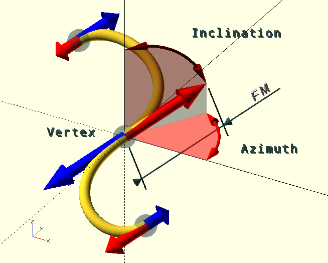
[[Vertex],[FM,INC,AZ],[{RM},{INC,AZ}]]
Example:
[[1,0,0],[1,90,90],[]] // The empty 'Reverse vector' (for default 'smooth' behaviour) is not strictly necessary here, but is inserted in conformance with the 3D convention (treated below), where it is required to enable standard indexing of the variables in the routines.Where:
-
[Vertex], vertex, the Tangent Point on the curve, at which point the tangent is known in two directions; forward along the curve and reverse. Unless it’s the first or the last TP in the set, the curve is split at the TP, i.e., the vertex is both the end-point of the previous partial curve and the start-point of the next.
It should be clear from the image that a curve does not have to be defined in any particular plane. Curves are 3D (objects).
The […M,INC,AZ] tuples are the
spherical coordinates
of the tangent vectors at the TP; one Forward (red in the image) and one Reverse (blue in the image). The curve in the image starts below Z=0, goes through the origin, and ends up somewhere in the (-++) octant, by the looks of it…
-
FM, scalar, the Forward Magnitude, or length of the forward tangent vector, or the distance to the adjacent control point in that direction, i.e., on the following (partial) curve segment.
-
INC, degrees [0,180], inclination of the forward tangent vector, i.e., the angle between the positive Z-axis and the direction in which the following curve segment leaves the tangent point.
-
AZ, degrees [0,360], azimuth of the forward tangent vector, i.e., the angle with the positive X-axis and the direction in which the following curve segment leaves the tangent point.
-
RM, scalar, the Reverse Magnitude, or length of the reverse tangent vector, or the distance to the adjacent control point in that direction, i.e., on the preceding (partial) curve segment.
-
INC, as above.
-
AZ, as above.
Each spherical coordinate defines the location of the adjacent Bézier curve control point, in its particular direction, relative to the TP Vertex.
Default behaviour is for smooth tangent points, i.e., the preceding curve segment arrives at a tangent point along the same tangent with which the following curve segment leaves. If the Reverse Magnitude RM is left undef, the FM value will be used.
If INC and/or AZ for the RM vector are left undef, the vector angles will be opposite to those of the FM vector, resulting in a smooth curve when both are left undef. If this is not the case, i.e., either INC or AZ or both are specified and not opposite to those of the FM vector, the curve will not be smooth, and have a 'kink' at the TP.
The Curve or Shape TPS and TPA
Even for a 'C'- or 'S'-shaped curve, you will need at least two tangent points, and for anything more complex, you may need several. They are put together in a TPS, or Tangent Point Set.
A TPS is a set of as many TP as you need, plus a Transforms record.
For more on the latter, see below, or the documentation at
TransformMatrix().
Here’s an example of a TPS for a quarter circle-arc with a radius of 10 units. It’s a bad example, because it has only two TP, and thus forms just a simple cubic Bézier curve:
function TPS_R10(Transforms=[])=
    [ // Tangent Point Set
        [ // Tangent Points
             [[10, 0,0],[5.52,90, 90],[]] // Reverse identical and smooth.
            ,[[ 0,10,0],[   0,90,180],[5.52]] // Reverse not identical, but smooth.
        ],
        Transforms
    ]
;
It’s convenient to express a TPS as a function; you can define a partial curve, in this case a quarter circle, and re-use it by moving it around with Transforms, sticking it together with other partial curves into a complex curve, which is what a TPA is, an example of which follows here. You can even generalise it by adding parameters turning values into factors, and use it for different helixes 'like wot I done below', heck, why not write a collection of (partial) curves…
HR=10; // Helix radius
HA=30; // Helix angle.
ZZ=tan(HA)*Pi*HR/2;  // Endpoint Z-coordinate
VM=HR*0.552/cos(HA); // Tangent Vector Magnitude

ST=Cycle(-30,30); // Animation.

// TangentPointSet
function TPS_R10(Transforms=[],FI=0,RI=0)=
    [
        [ // Tangent Points
             [[HR, 0, 0],[VM,90-HA+FI,90],[0,undef,undef]]
            ,[[ 0,HR,ZZ],[ 0,0,0],[VM,90+HA-RI,0]]
        ],
        Transforms
    ]
;

// TangentPointArray
TPA=[   // Re-use the same TPS 4x.
         TPS_R10([              [0,0,   0,"T"]])
        ,TPS_R10([[0,0, 90,"R"],[0,0,  ZZ,"T"]])
        ,TPS_R10([[0,0,180,"R"],[0,0,2*ZZ,"T"]],0,ST)
        ,TPS_R10([[0,0,270,"R"],[0,0,3*ZZ,"T"]],ST,0)
    ]
;

BezierCurve(TPA,30,0.2);|
|
Even if there is only one TPS, it must be enclosed in square brackets to form a TPA like this: TPA=[TPS], so BezierCurve() doesn’t stumble; it always expects a TPA, (or a CPA, CPS, or CP).
|
How Shapes are unlike Curves.
A shape TP is identical to the curve TP above, so much so that The GHOUL won’t complain if you call BezierCurve() and BezierShape() with the same TPA, however, the behaviour of the two routines is somewhat different, and so are the results.
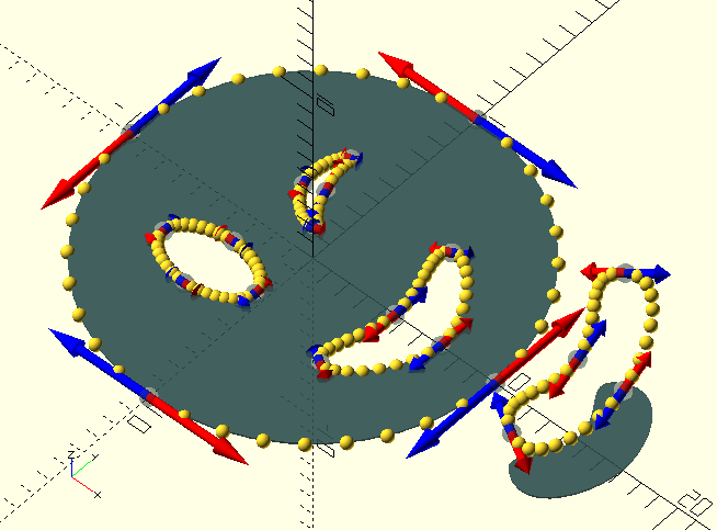
Since shapes are 2D polygons, to be used with linear_extrude(), any 3D aspect in the spherical coordinates or 'curvature vectors' is removed by projecting them onto the Z=0 plane, effectively rendering the resulting 'shape-curve' 2D, after which the vertices are cropped, i.e., the Z coordinates—now equal to 0—are removed, leaving a true 2D result. In short, a shape TPS should have an empty Transformations record, and 90 degree inclinations, else, your magnitudes will become projections of magnitudes, and their scalar value may no longer be what you expect; unless you’re expecting the
unexpected.[4]
The 'displaced smile' in the image is an example of what I’m talking about here; the curve is 'floating' above Z=0, but the resulting shape is its projection. I apologise for the sinister vibes of my attempt at a 'winky face'…
The second difference between shapes and 'regular' curves—with respect to The GHOUL’s Bézier functions—is that shapes must, by necessity, be closed curves, and BezierShape() forces this behaviour, ruthlessly, with callous disregard for your intentions, and without the merest consideration for the potential fallout of its perfunctory actions. Consider yourself warned.
Finally, BezierCurve() interprets each TPS as the 'next part of the curve', but in shapes, each TPS is considered a separate, closed path (forming a polygon), and—similar to the OpenSCAD convention for polygons—they are subtractive when they overlap.
The 3D solid TP, TPS and TPA
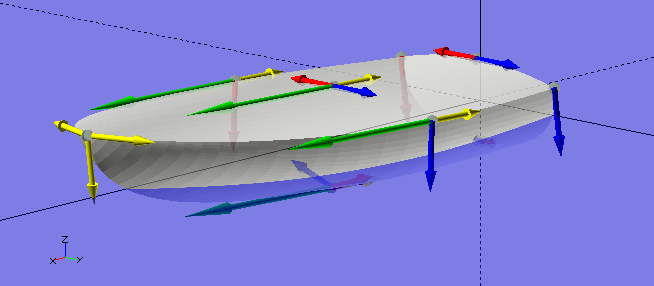
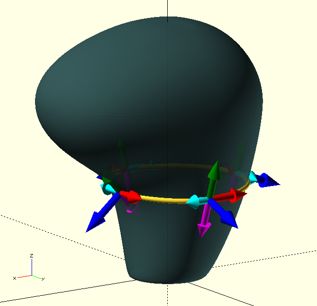
In The GHOUL, Bézier definitions of 3D solids are essentially a collection of cross-sections through the solid. Sets of tangent points form 2D slices, and several of these are 'stacked' to form the solid, after which a 3D mesh is generated for the polyhedron(). Clearly, we need to define the curvature, not just around the 2D slices, but also between the individual slices. in order to achieve this, each TP contains not two but four tangent vectors; two for the forward and reverse curvature around the slice (red and blue in the image), one for the curvature towards the next slice (green), and one for the curvature towards the previous slice (yellow).
|
|
The boat here was my first attampt at a 3D solid, defined by a TPA, and it surprised me how easy it is to define a solid, and with so few data-points. It’s magic, all thanks to Messrs. Bézier and de Casteljau. Here's the source code for that super-snazzy boat in the image, as well as some beautiful prose by John Ruskin, and perhaps you’d like to have a look at a short (1 min.) OpenSCAD screen-grab video of it here. Watch to the end, you’ll like it, I promise… |
As for the 3D TPS and TPA, what goes for curves and shapes applies here too, there’s no sense in rehashing; have a look back there if you need to. Each TPS defines a cross section through the solid, starting at the 'bottom'. A TPS is generally defined on Z=0 before being moved to its 'place proper' by the Transforms. The TPA contains all TPS cross sections, forming the solid.
The basic form of a 3D TP is:
[[Vertex],[FM,INC,AZ],[{RM},{INC,AZ}],[NM,INC,AZ],[{PM},{INC,AZ}]] // {} parameters are optional.
Example:
[[1,0,0],[1,90,130],[],[2,10,0]] // The empty 'Reverse vector' (for default 'smooth' behaviour) may NOT be omitted, in order to maintain standard indexing of the parameters (how else would the routines know this is a 3D *TP*), the 'Previous (slice) vector' can and has been omitted, so 'vertical' curvature will also be smooth.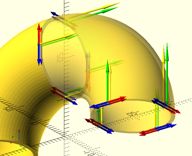 And to give you an example of what not to do, or how two lines of code are better than twenty, here’s a Bézier-based 3D solid 'elbow', and its
 rotate_extrude() counterpart. There are times you need Bézier curves, and there are times when you really don’t. Bézier curves are not for defining 'regular shapes', by which I mean shapes easily described by regular functions like circles, ellipses, cones &c.
Irregular shapes like boats and torsos, however, gear-shift knobs, organic shapes; that’s where Bézier curves shine. Still, the below example does illustrate quite well how a TPS can be parametrized and re-used in a TPA to form a more complex solid. Have a gander at the code, how not to define a 90 degree elbow, and how to do it right (in the last two lines)…
function TPS_R(Transforms=[],R=10,RB=20,NM=1,PM=0,NI=0,SRO)=
    [ // Tangent Point Set (a closed curve cross-section)
        [ // Tangent Points, forming a circle.
             [[ R-RB,   0,0],[0.552*R,90, 90],[],[0.552*(RB-R)*NM,NI,0],[0.552*(RB-R)*PM]]
            ,[[  -RB,R,0],[0.552*R,90,180],[],[  0.552*(RB)*NM,NI,0],[  0.552*(RB)*PM]]
            ,[[-R-RB, 0,0],[0.552*R,90,270],[],[0.552*(RB+R)*NM,NI,0],[0.552*(RB+R)*PM]]
            ,[[  -RB,-R,0],[0.552*R,90,  0],[],[  0.552*(RB)*NM,NI,0],[  0.552*(RB)*PM]]
        ],
        Transforms,SRO // SRO, Set Resolution Override, e.g., smaller resolution for close spaced sets. In this case the 'cut surface' at the end of the elbow.

    ]
;

function TPA(R=10,W=1,RB=20,SRO=4)=[
    TPS_R([],R,RB,1,0,0),
    TPS_R([[0,90,0,"R"]],R,RB,0,1,0,SRO),
    TPS_R([[0,90,0,"R"]],R-W,RB,1,0,180),
    TPS_R([],R-W,RB,0,1,180,SRO)
];

ShowTPA(TPA());
color(OSG,0.5)
BezierSolid(TPA(),30,30,Doughnut=true);

rotate([90,0,0])
Torus(20,90)
Ring(10,1,Centered=true);
The routines
BezierVertex()
Not that you’re likely to ever need BezierVertex(), which, by the way, is an alias for DeCasteljau() (so use that if you ever need to, The GHOUL does).
It really is a 'non-user-background-routine', but I’d like to have a quick look at it here, for completeness' sake, because it may shed some light, and, well, it’s logical to start there.
BezierVertex(CPS, Fraction)
-
CP, Bézier curve Control Polygon, an array of—usually—four vertices.
-
Fraction, fraction [0,1] of the curve, where the vertex lies.
BezierVertex() returns the coordinates for the point at Fraction on the Bézier curve defined by the CP, see the code block below for an example.
BezierVertex.scad also contains CBezierVertex() and QBezierVertex(), the Bernstein polynomial forms for cubic and quadratic Bézier curves.
Finally—and stay away from this one please, I mean it—it contains GenBezierVertex(), the general Bernstein polynomial form, which is frighteningly computationally expensive; your GPU will hate you.
// A cubic Bezier curve approximation of a quarter circle.
function CP(Radius)=[[1, 0, 0], [1, 0.552, 0], [0.552, 1, 0], [0, 1, 0]]*Radius;
// The curve vertex.
V=BezierVertex(CP(10),0.75);
translate(V)
sphere(r=0.5);
You might perhaps do something akin to what
BezierTransitionUp()
does, using BezierVertex(), or better, CBezierVertex(), with some fancy curve-shape of your own; have a look at the documentation
there,
and the library file TheGHOUL/Lib/Bezier/BezierVertex.scad.
BezierCurve()
|
|
Like some other of The GHOUL’s routines, there is a function and a module version of this routine, however, unlike most cases, the |
The function
BezierCurve(TPA, Resolution)
-
TPA, Tangent Point Array—an array of Bézier tangent point sets—or a Control Polygon Set.
-
Resolution, integer, curve resolution, a bit like OpenSCAD’s $fn.
BezierCurve() takes either a TPA—see the
conventions
above—or a CP or CPS, a (set of) Bézier control polygon(s). For simple curves, a CP(S) is simpler and perhaps faster to 'construct' than a TPA.
CP=[[10,0,0],[10,5.52,0],[5.52,10,0],[0,10,0]]; // A Bezier control polygon.
BezierCurve(CP,30);
color(BLU){
ShowCurve(CP,0.2,1,false); // Control polygon points.
ShowCurve(CP,0.05,1,true); // Control polygon 'curve'.
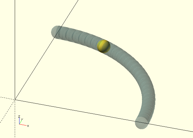
}For more complex curves, the TPA is definitely superior, especially when it comes to 3D control of complex curves. A TPA is an array of tangent point sets. Two tangent points describe the cubic Bézier curve between them, so each set contains at least two tangent points, describing a partial curve—see the code block and full description below.
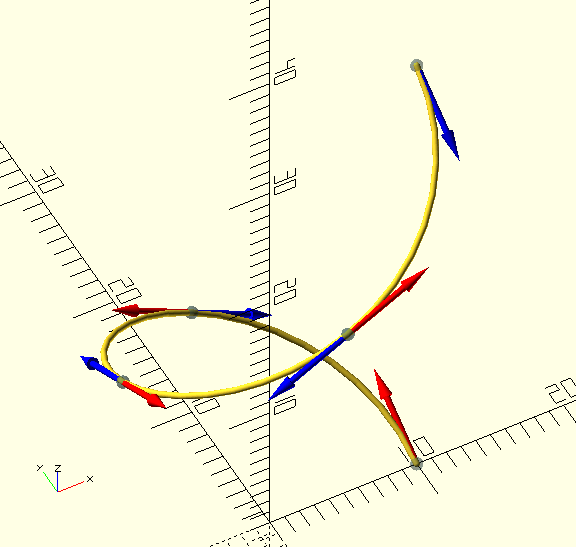
Let’s look at the definition of a helical curve. Only a 90 degree portion of the helix is described by the TPS, but the TPA grabs it four times, each time feeding the TPS a Transforms parameter with the translation and rotation required to move it into position so the endpoints coincide, and a smooth, continuous curve is created.
See TransformMatrix() for documentation about the Transforms used here.
In the image, the tangent points are the grey spheres, the 'forward' magnitudes are the red vectors, and the 'reverse' magnitudes are blue. The source file is TheGHOUL/DemoFiles/Img_BezierCurve.scad.
HR=10; // Helix radius
HA=30; // Helix angle.
ZZ=tan(HA)*Pi*HR/2;  // Endpoint Z-coordinate
VM=HR*0.552/cos(HA); // Tangent Vector Magnitude

function TPS_R10(Transforms=[])=
    [ // TangentPointSet
        [ // Tangent Points
             [[HR, 0, 0],[VM,90-HA,90],[0,undef,undef]]
            ,[[ 0,HR,ZZ],[ 0,0,0],[VM,90+HA,0]]
        ],
        Transforms
    ]
;

// TangentPointArray
TPA=[   // Re-use the same TPS 4x.
         TPS_R10([              [0,0,   0,"T"]])
        ,TPS_R10([[0,0, 90,"R"],[0,0,  ZZ,"T"]])
        ,TPS_R10([[0,0,180,"R"],[0,0,2*ZZ,"T"]])
        ,TPS_R10([[0,0,270,"R"],[0,0,3*ZZ,"T"]])
    ]
;

// See TheGHOUL/Lib/Matrices/TransformMatrix.scad for documentation about the 'Transforms' used here.

BezierCurve(TPA,30,0.2);
The module
BezierCurve(TPA, Resolution, Radius, Frac, Connect, Closed)
The BezierCurve() function is meant for generating curves or paths to generate objects with, it creates lists of vertices, not objects. But maybe you do want a 'curve-object' (I just did), so there’s the module… It’s really just the BezierCurve() function and
ShowCurve()
module wrapped up in one, which is why it takes most of the parameters that those routines take…
Yes, you could probably just as easily do ShowCurve(BezierCurve()), but then, you probably do know about my penchant for writing identically named functions and modules by now…
BezierShape()
To generate a polygon that is in part or entirely made up from Bézier Curves with The GHOUL, you have a few options:
-
Generate it by hand. As if.
-
Call
BezierCurve()(multiple times), and callpolygon()with the resulting vertex array(s) and path(s). Not ideal. -
Use
SVG()to generate it [5]. You’ll probably end up working with Bézier curves again anyway, but it’s certainly a good alternative (which you may prefer) to: -
Call
BezierShape()with a TPA. And be done. It even interprets multiple paths correctly…
BezierShape(TPA,Resolution)
-
TPA, a tangent point array.
-
Resolution, curve resolution.
In the image, the actual shape is rendered in DarkSlateGrey, and for clarity, the actual vertex arrays as well as the tangent points and tangent vectors are displayed.
When the TPA contains more than one TPS, additional paths are subtracted from the shape where/if they overlap, in analogy with OpenSCAD’s polygon(), after all, creating a linear_extrude()able polygon is exactly what this routine does.
There is also a BezierShape() function, which returns the shape—as per The GHOUL’s convention—in a tuple of vertices and paths: [[Vertices],[Path(s)]].
R=10;
VL=R*0.552;
/* The documentation image. */
function Shape0()=
    [
        [[ // Main shape.
            [[ R, 0,0],[VL,90, 90]],    // P0
            [[ 0, R,0],[VL,90,180]],    // P1
            [[-R, 0,0],[VL,90,270]],    // P2
            [[ 0,-R,0],[VL,90,  0]]     // P3
        ],[]],
        [[ // Smile.
            [[  7, 0,0],[2,90, 90]],    // P0
            [[  4, 4,0],[1,90,210]],    // P1
            [[4.5, 0,0],[2,90,270]],    // P2
            [[  4,-4,0],[1,90,330]]     // P3
        ],[]],
        [[ // 'Displaced' smile.
            [[  7, 0,0],[2,90, 90]],    // P0
            [[  4, 4,0],[2,90,210]],    // P1
            [[4.5, 0,0],[2,90,270]],    // P2
            [[  4,-4,0],[2,90,330]]     // P3
        ],[[30,0,0,"R"],[10,0,5,"T"]]],
        [[ // Winky eye.
            [[  0, 0,0],[  2,90, 90]],  // P0
            [[0.3, 2,0],[0.5,90,180]],  // P1
            [[ -1, 0,0],[  1,90,270]],  // P2
            [[0.3,-2,0],[0.5,90,  0]]   // P3
        ],[[0,0,20,"R"],[-2,3,0,"T"]]],
        [[ // Open eye.
            [[ 2.5,   0,0],[1,90, 90]], // P0
            [[   0, 1.5,0],[1,90,180]], // P1
            [[-2.5,   0,0],[1,90,270]], // P2
            [[   0,-1.5,0],[1,90,  0]]  // P3
        ],[[-3,-3,0,"T"]]]
    ]
;

// Vectors
ShowTPA(TPA);

// The shape itself
color(DSG,0.7)
linear_extrude(0.1)
BezierShape(TPA,10);

// The curve vertices--how cool is this?
// All Bézier routines can digest the same TPA :-)
BezierCurve(TPA,10,true,true,0.3,1,false);
BezierSolid()
Solids are defined by a TPA, an array of Tangent Point Sets, just as curves and shapes are. Each TPS forms a cross-section through the solid, also referred to as a 'plane'. The tangent points have a second Tangent Vector pair, pointing to the previous plane and the next plane, to define curvature in the '3D direction'.
`BezierSolid(TPA,SectionResolution,SetResolution,EndCaps,Closed,Doughnut)
-
TPA, Tangent Point Array—an array of Bézier tangent point sets—or a Control Polygon Set.
-
SectionResolution, integer, resolution of the curves around each cross section, a bit like OpenSCAD’s $fn.
-
SetResolution, , integer, resolution of the curves between two cross sections.
-
EndCaps, Boolean, the solid is 'capped' on both ends if true.
-
Closed, Boolean, the solid is 'slit' lengthwise if false.
-
Doughnut, Boolean, the top of the solid is connected to the bottom, as a closed 'pipe' or a doughnut if true.
To generate a Bézier polyhedron, or 3D solid with The GHOUL, you must:
-
Know what your polyhedron is supposed to look like.
-
Create a Tangent Point Set or TPS for each cross-section, at optimal locations in the polyhedron.
-
Combine the TPS into an array called a TPA.
-
Call
BezierSolid()with the TPA as it’s parameter. This is the only call you need to make.
How do you do all that? It’s a long story, and it’s easier to show you:
A worked example
Enough of all the talk. Subject matter like this is best learned by going through an example, so here it is: We’re going to design a heart-shaped ring-box—just in case you’re reading this around the beginning of February.
|
|
Tangent Points should be placed where the curvature of the object changes, in a solid, this means either 'circumferential' curvature changes, or 'longitudinal' curvature changes. |
Just like when you give a person directions to your house, you don’t tell them "go straight, then keep going straight, go straight some more", you tell them "turn right at the candy store, left at the lights, then right at the green house and you’re there". Change is what matters.
The next thing to remember is that a cubic Bézier Curve is excellent at describing a 90 degree turn, pretty good at describing an s-bend or even a half turn, but crappy at anything like a three-quarter turn; you’ll need to split that curve, define another Tangent Point.
|
|
Whenever the curve of a body turns over 90 degrees, you will probably need another Tangent Point, if it turns over 180 degrees, you will need another, unless you’re lucky and like the funky curves you’ll get. |
|
|
Tangent Points must be placed wherever the location and/or curvature of the object needs to be defined accurately. |
Okay, let’s see what we’re aiming for here: A heart shaped box with a flattened bottom. It’s just the basic shape we’re after, I’m not going to cut it into a box part and a lid, or add hinges or whatever; it’s only Feb. 3rd, you have plenty of time for that.
The big changes in curvature of a basic heart-shape happen obviously at the point and the valley between the two lobes, so we’ll need some TPs there. How about the lobes themselves? Will we need two TPs per lobe or will one be enough? This choice comes down to how accurately we want to approximate a true half circle.
Tangent Points
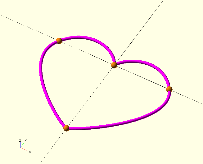
I think we’re after the general shape here, not some accurate machine part, so we’re going with the KISS-principle and use only one TP per lobe:
This gives us a total of four TP, see the image.
In the rest of this example, we’ll refer to the four TP in the image as TP0…TP3. TP0 is on the X-axis, TP1 is on the origin and so on.
Have another look at the Curve TP if you need a refresher on the TP parameters. What’s important to remember here is the additional two sphericals for the curvature vectors pointing to the next cross section, NM, and the previous cross section, PM. They have the same structure as their 2D counterparts. As we’ve seen earlier, a basic 3D TP looks like this:
TP=[[Vertex],[FM,INC,AZ],[{RM},{INC,AZ}],[NM,INC,AZ],[{PM},{INC,AZ}]];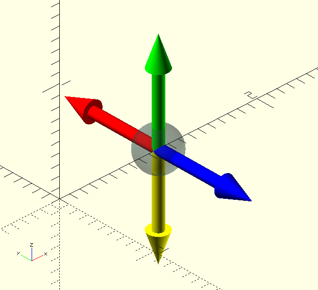
Typically, a TP will initially have the Magnitudes set to 1 with the spherical curvature vectors in the standard orthogonal directions, an Inclination of 90 is usually a good staring point for the forward and reverse vectors, and .
A starting TP, somewhere on the positive X-axis, with the forward Curvature Vector pointing along Y+, a smooth reverse CV, i.e., pointing along Y-, the 'next' CV pointing up along Z+, and a smooth 'previous' CV, pointing down along Z- would look like this:
TP_=[[X,0,0],[1,90,90],[1],[1,0,0],[1]];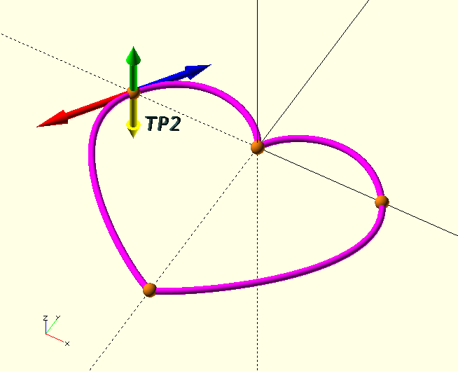
In the image, the TP curvature vectors for TP2 are displayed. Remember that each TP is at the same time the end-point (P3) of the previous curve and the start-point (P0) of the next curve. The yellow vector points at the adjacent control point on the previous cross section, and the green vector points at the adjacent control point on the next cross section.
Let’s Set up this Tangent Point Set.
The Tangent Point Set
We need four tangent points with coordinates [20,0,0], [0,0,0], [-20,0,0] and [0,-30,0]. We’ve seen the general structure for a TP already, but a TPS is a little more involved. A TPS is given in the form of a function, this has two big advantages:
-
We can use the same TPS several times at different places in the polyhedron by specifying different Transform parameters.
-
We can replace certain values with parameters so we can easily change the TPS.
We’ll get back to the Transform parameters below. They are also treated more in depth in the entry for
TransformMatrix()
function Heart(
Transforms=[[0,0,0,"T"]]
)=
[
[
[[ 20, 0,0],[1,90, 90],[],[1,0,0]],
[[ 0, 0,0],[1,90,180],[],[1,0,0]],
[[-20, 0,0],[1,90,270],[],[1,0,0]],
[[ 0,-30,0],[1,90, 0],[],[1,0,0]]
],
Transforms
]
;
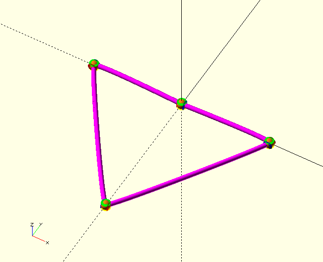
ShowTPA([Heart()],Sets=undef,Points=undef,Vectors=undef,Curves=undef,Closed=true,Radius=1,Thickness=1,Resolution=30,Connect=true,CColor=MGT,PColor=CPR);Because the curvature vectors lengths are still at 1, the result (shown in the image below) is not too impressive. Before we change that, however, let’s have a look at that last call, ShowTPA() is a module that—nomen est omen—shows the elements of a TPA, and is very useful for troubleshooting.
Note that the TPS needs to be [bracketed] to become a TPA.
ShowTPA()
ShowTPA(TPA,Sets=undef,Points=undef,Vectors=undef,Curves=undef, Closed=true,Radius=1,Thickness=1,Resolution=30, Connect=true,CColor=MGT,PColor=CPR)
-
TPA, Tangent Point Array, or a bracketed TPS
[TPS]. -
Sets, Tuple, only the specified TPS are shown. If left undef, all are shown. This behaviour is the same for all pameter tuples in this module.
-
Points, Tuple, only the specified Tangent Points are shown.
-
Vectors, Tuple, only the specified Vectors are shown.
-
Curves, Tuple, only the specified Curves are shown.
-
Closed, Boolean, for closed/sliced 3D solids.
-
Radius, Scalar, tangent point sphere radius.
-
Thickness, Scalar, curve and vector diameter.
-
Resolution, Integer, curve resolution, similar to $fn.
-
Connect, Boolean, curve vertices are connected if true.
-
CColor, PColor, Colors for curves and tangent points.
Let’s give those curvature vectors something to do. Start with values of around 0.2 to 0.5 times the distance between the tangent points.
function Heart(
        Transforms=[[0,0,0,"T"]]
    )=
    [
        [
            [[ 20,  0,0],[10,90, 90],[],[1,0,0]],
            [[  0,  0,0],[10,90,180],[],[1,0,0]],
            [[-20,  0,0],[10,90,270],[],[1,0,0]],
            [[  0,-30,0],[10,90,  0],[],[1,0,0]]
        ],
        Transforms
    ]
;
Better, but not what we’re after yet. When we look at the image, it’s clear that the curvature vectors are’t tangential to the shape we’re after. We’ve set the Inclination of all vectors to 90 degrees, which puts them in the Z=0 or X-Y plane. The TP3 (the 'tip' of the heart) tangent vector has an Azimuth value of 0 (+X-axis) which makes sense because, being on the mid-line of a symmetrical shape, the tangent there is horizontal. The tangent vectors of TP0 and TP2, however, have Azimuth values of 90 and 270 which puts the tangents there in the vertical, which is clearly incorrect, and TP1 (the 'valley') clearly needs tangent vectors that are not inline, to get the sharp change of direction it needs. The Magnitudes of the vectors probably also need some 'tuning'.
Here are the new values:
function Heart(
        Transforms=[[0,0,0,"T"]]
    )=
    [
        [
            [[ 20,  0,0],[12,90,125],[15      ],[1,0,0]],
            [[  0,  0,0],[ 6,90,115],[ 6,90,65],[1,0,0]],
            [[-20,  0,0],[15,90,235],[12      ],[1,0,0]],
            [[  0,-30,0],[ 2,90,  0],[        ],[1,0,0]]
        ],
        Transforms
    ]
;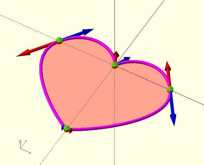
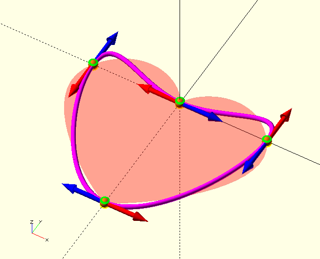
That’s the ticket. Check out TP0, the right one in the image. See where the tangent vector is pointing? As mentioned already, it has an inclination of 90 degrees to bring it from aligned with the positive Z-axis down to the X-Y plane, then it has an azimuth, the angle with the positive X-axis, of 125°. TP3 was fine already, but to get a smaller radius of curvature at the tip, the vectors have been given a magnitude of only 2. TP2 has the 'mirror' value of TP0, 235°. To get a nice balanced shape at the lobes, the magnitudes going 'up the lobe' to the valley (the smaller distance) are slightly smaller than the ones going 'down' to the tip, which, with a bigger distance to cover, need to have a larger radius. TP1 is a bit 'special', since it describes a sharp 'corner', its vectors are not aligned, and instead each points along the direction with which the curve arrives (from 65°) and depart (to 115°) the vertex.
Take a moment to study the image and the respective tangent points in the code above, until the make sense to you.
Suppose for a moment that all we want is a polygon of this shape…
color(RED)
linear_extrude(10)
BezierShape([Heart()]);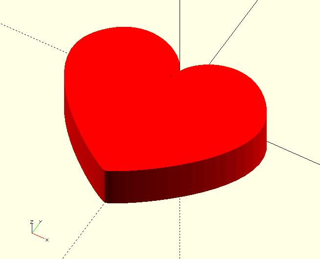
All you need is the TPS—in [brackets] to become a TPA—and one call.
Pretty nifty, but we want a fancy box, so we’ll use this TPS in the next section as the basis of a set of TPS; a TPA (Tangent Point Array).
Making a Tangent Point Array
A 'Transforming' Intermezzo
As we’ve seen, Tangent Point Sets are declared as a function to allow for parameters to be used in the TPS definition, which makes it easier to re-use the TPS at different locations in the polyhedron. Working with the Transform parameter, we can re-use the same same TPS to make our Tangent Point Array, but this heart-shaped box isn’t the best example for that; we need three very different TPS, so we’ll design those, based on the one we’ve already got. We do use the Transform parameters to position these TPS in the polyhedron, so let’s have a quick intermezzo and look at them now.
function Your_TPS_Name(
    Transforms=[[0,0,0,"T"]],  // Section transformations (translate/rotate &c.)
    Foo=10, Bar=5              // Some variable dimensions, these can represent
                               // coordinates, inclination and azimuth or
                               // lengths of vectors &c.
    )=
    .
    .
    .
;
Because the TPS (cross section of the polyhedron) is always defined on the Z=0 plane, it needs to be moved to it’s proper location. The 'Transforms' in the function declaration are those transformations that bring the cross section to it’s position within the polyhedron or 3D space, formatted as three numbers plus a one letter string, "T", "S" or "R" for Translate, Scale, and Rotate, for example:
[[0,0,10,"T"],[1,1,-1,"S"],[0,0,180,"R"]]They are interpreted in the usual OpenSCAD way (X-Y-Z units and degrees) and are performed in left to right order. See the
TransformMatrix()
function entry for a more in-depth discussion.
|
|
A Tangent Point Set can be used several times in the same polyhedron, simply rotate, translate or even scale the TPP and re-use it in a different location without the need to define it again. |
Multiple TPP are then combined into a TPA and processed into a polyhedron like this:
Heart=
[
    Bottom([[0,0,0,"T"]]),
    Middle([[0,0,10,"T"]]),
    Middle([[1.2,1.2,1,"S"],[0,0,15,"T"]]),
    Middle([[0,0,20,"T"]]),
    Top([[0,0,30,"T"]])
];

BezierSolid(Heart,30);
Back to the job in hand…
To create our TPA, we take the following steps:
-
Use the TPS we have for the middle of the box.
-
Use the same TPS we have for the bottom but:
-
Make it smaller.
-
Move it towards the center.
-
-
Make a new TPS for the top of the box, this TPS:
-
Must be very small.
-
Also needs to be centered.
-
In addition to that, we need to give some thought to the vectors pointing 'vertically' from one cross section to the next. Let’s dive in:
function HeartBottom(
        Transforms=[[0,0,0,"T"]]
    )=
    [
        [ // Note smaller size, otherwise unchanged from middle section.
            [[ 10,  0,0],[12,90,125],[15      ],[1,0,0]],
            [[  0,  0,0],[ 6,90,115],[ 6,90,65],[1,0,0]],
            [[-10,  0,0],[15,90,235],[12      ],[1,0,0]],
            [[  0,-15,0],[ 2,90,  0],[        ],[1,0,0]]
        ],
        Transforms
    ]
;

function HeartMiddle(
        Transforms=[[0,0,0,"T"]]
    )=
    [
        [
            [[ 20,  0,0],[12,90,125],[15      ],[1,0,0]],
            [[  0,  0,0],[ 6,90,115],[ 6,90,65],[1,0,0]],
            [[-20,  0,0],[15,90,235],[12      ],[1,0,0]],
            [[  0,-30,0],[ 2,90,  0],[        ],[1,0,0]]
        ],
        Transforms
    ]
;

function HeartTop(
        Transforms=[[0,0,0,"T"]]
    )=
    [
        [ // Note MUCH smaller size, otherwise unchanged from middle section.
            [[ 2, 0,0],[12,90,125],[15      ],[1,0,0]],
            [[ 0, 0,0],[ 6,90,115],[ 6,90,65],[1,0,0]],
            [[-2, 0,0],[15,90,235],[12      ],[1,0,0]],
            [[ 0,-2,0],[ 2,90,  0],[        ],[1,0,0]]
        ],
        Transforms
    ]
;

/*
  Put it all together into a single solid.
  Note the transforms move the section to its 3D location.
*/
Heart=
[
    HeartBottom([[0, -5,-10,"T"]]),
    HeartMiddle([[0,  0,  0,"T"]]),
    HeartTop(   [[0,-10, 10,"T"]])
]
;

BezierSolid(Heart);
Yikes. There are a few problems here, the bottom is distorted, and the edge in the middle is sharp, not nice and rounded.
The first issue is caused by the curvature vectors that are much too big for the reduced size of the bottom, causing the curve to 'overshoot'. The solution is simple; make them smaller.
The second issue is not hard to solve either, the 'Z-direction' curvature vectors pointing to the 'Bottom' TPS and 'Top' TPS are very small, this small curvature results in the curve immediately turning towards the other sections instead of curving slowly that way; so we make them bigger.
Here are the changes:
function HeartBottom(
        Transforms=[[0,0,0,"T"]]
    )=
    [
        [ // Note smaller curvature vector magnitudes compared to middle section. Also, the vectors pointing to the next and previous section.
            [[ 10,  0,0],[7,90,125],[5      ],[3,90, 60],[0]],
            [[  0,  0,0],[3,90,115],[3,90,65],[3,90, 90],[0]],
            [[-10,  0,0],[5,90,235],[7      ],[3,90,120],[0]],
            [[  0,-15,0],[1,90,  0],[       ],[9,90,270],[0]]
        ],
        Transforms
    ]
;

function HeartMiddle(
        Transforms=[[0,0,0,"T"]]
    )=
    [
        [ // Note the vectors pointing to the next and previous section.
            [[ 20,  0,0],[12,90,125],[15      ],[10,0,0]],
            [[  0,  0,0],[ 6,90,115],[ 6,90,65],[10,0,0]],
            [[-20,  0,0],[15,90,235],[12      ],[10,0,0]],
            [[  0,-30,0],[ 2,90,  0],[        ],[ 6,0,0]]
        ],
        Transforms
    ]
;

function HeartTop(
        Transforms=[[0,0,0,"T"]]
    )=
    [
        [ // Note MUCH smaller curvature vector magnitudes compared to middle section. Also, the vectors pointing to the next and previous section.
            [[ 2, 0,0],[1,90,125],[1      ],[0,0,0],[10,90, 35]],
            [[ 0, 0,0],[1,90,115],[1,90,65],[0,0,0],[ 6,90, 90]],
            [[-2, 0,0],[1,90,235],[1      ],[0,0,0],[10,90,145]],
            [[ 0,-2,0],[1,90,  0],[1      ],[0,0,0],[15,90,270]]
        ],
        Transforms
    ]
;

Heart=
[
    HeartBottom([[0, -5,-10,"T"]]),
    HeartMiddle([[0,  0,  0,"T"]]),
    HeartTop(   [[0,-10, 10,"T"]])
]
;

BezierSolid(Heart);
Here it is. All done. Go ahead and 'right click' on the image to view it larger, it’s probably worth it.
Take a good look at the curvature vectors between the TPS sections; see how the 'bottom' section has 90° inclinations, pointing to the 'middle' section, causing the curve to be tangent to Z=0. Also look at the 'top' section, where the same applies, but for the vectors pointing back at the 'middle'.
Look at the individual curvature vectors and the local shape of the polyhedron, see the correlation.
Go back over the incremental changes to see what effect each has. When I get the time, I’ll add some more examples and images below.
The full code for all the images is in the file TheGHOUL/DemoFiles/WorkedExample.scad, go mess with it and see how the changes affect the shape, and get a feel for things. I hope you’ll find Bézier curves—and this library—as satisfying to work with as I do.
There’s more
These are the remaining Curves Library routines. Not all are involved with Bézier Curve generation, some only provide information, some are helpers for other routines.
BezierFractionX()
BezierFractionX(ControlPoints, X, Precision)
-
ControlPoints, a set of Bézier Curve Control Points
-
X, scalar, the coordinate to search.
-
Precision, scalar, the required precision.
BezierFractionX() finds the Fraction of a point on the Bézier Curve that will result in an X-coordinate within Precision of X, when Fraction is used in the de Casteljau algorithm. The de Casteljau algorithm uses a fraction to find a point on a Bézier Curve, this routine is kind of a 'reverse de Casteljau'.
BezierFractionY()
BezierFractionY(ControlPoints, Y, Precision)
-
ControlPoints, a set of Bézier Curve Control Points
-
Y, scalar, the coordinate to search.
-
Precision, scalar, the required precision.
BezierFractionY() is the 'Y-variant' of BezierFractionX() above.
BezierCurveLength()
BezierCurveLength(ControlPoints, Fraction, Resolution)
-
ControlPoints, vertices, Bézier Curve control points.
-
Resolution, integer, the curve’s resolution, i.e., the number of vertices in the finished curve.
-
Fraction, fraction [0,1] of the curve, see comment at
BezierFractionX().
Returns the developed length of the curve or curve fraction if Fraction<_1_.
Essentially a 'shorthand version' of CurveLength(BezierCurve()) in it’s own right (it uses neither routine).
DeCasteljau()
DeCasteljau(ControlPoints, Fraction)
-
ControlPoints, vertices, Bézier Curve control points.
-
Fraction, fraction [0,1] of the curve at which to find the vertex, see comment at
BezierFractionX().
An implementation of the most marvellous algorithm developed by Mr Paul de Casteljau.
See
BezierVertex().
ShowDeCasteljau()
ShowDeCasteljau(BezierSet, Fraction, Resolution)
-
BezierSet, array of on or more sets of Bézier Curve control points.
-
Fraction, fraction [0,1] of the curve at which to find the vertex, see comment at
BezierFractionX(). -
Resolution, integer, the curve’s resolution, i.e., the number of vertices in the finished curve.
ShowDeCasteljau() is only useful for visualising the generation of a Bézier Curve.