Old Vespas are very appealing to me. I love the way they feel. I love the way they smell. I love the curves on them.
|
|
All 'Curve objects' in The GHOUL are nothing but 'lines' or curves with a cylindrical cross-section, even if the are 'in a 2D plane'. In The GHOUL, the 'resolution', or the number of segments—also called 'fragments' in OpenSCAD documentation—of the cross-section of the curve object itself, is determined only by The GHOUL’s own special variable $fc, (i.e. fragments of curve elements) while in this respect $fn (i.e. fragment number) is entirely ignored. If $fc=0,
Segments() is used to determine the appropriate segment number.
|
This is the home of general curves. Bézier curves, and SVG curves and shapes, have their own pages. Some of the routines here are not necessarily curve 'generators', but may be so 'curve specific' that they really aren’t at home (any better) anywhere else, and thus reside here.
Circles and Arcs
|
|
Arcs are not circles. The following routines started out as one, but an arc has an endpoint, and a circle doesn’t. There’s no such thing as a 360 degree arc; an arc is part of a circle. "So what, who cares about linguistics? We’re 3D modelling here!" you say. Well, as with everything; if it’s worth doing, it’s worth doing it right, and this difference becomes essential when generating lists of vertices, as the endpoint of a 360 degree arc would overlap the starting point. So, there’s a reason 'in principle', as well as a practical one. It also makes for clearer code—IMNSHO—which is a bonus. |
Arc()
The Function
Arc(StartAngle,EndAngle,Radius,FullEnds=true,3D=false)
-
StartAngle, angle in degrees [0, 360] where the arc starts.
-
EndAngle, angle in degrees [0, 360] where the arc ends.
-
Radius, dimension, radius of the arc.
-
FullEnds, Boolean, if true, the arc 'n-gon' has endpoints with radius=Radius.
-
3D, Boolean, if true, vertices will receive 3 coordinates (with Z=0).
The Arc() function returns a list of vertices forming an arc.
Arcs and circles are really n-gons, made up of segments. By default, when the endpoints are somewhere between two of the n-gon corners, they are at full Radius. This gives 'deformed' ends to the n-gon arc, however, they join up with tangential lines to the 'theoretical' curve in that point, which is behaviour an unsuspecting user might expect…
If FullEnds=false, start and end points, regardless of whether they lie on a proper n-gon corner point, or somewhere in between, are located on the segment line proper, i.e., we’re literally cutting a segment from the n-gon, preserving the endpoint positions on the segment line, as well as the angular relationships between the line segments.
The Module
Arc(StartAngle, EndAngle, Radius, Thickness, Pattern=undef, FullEnds=true)
-
StartAngle, angle in degrees [0, 360] where the arc starts.
-
EndAngle, angle in degrees [0, 360] where the arc ends.
-
Radius, dimension, radius of the arc.
-
Thickness, dimension, diameter of the 'drawn' curve.
-
Pattern, Tuple, dash-dot pattern in unit line lengths.
-
FullEnds, Boolean, if true, the arc 'n-gon' has endpoints with radius=Radius.
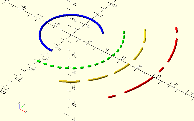
The Arc() module 'draws' an arc; it’s used in images to indicate pitch-circles and such. To get a dashed or dotted line, specify the pattern as a tuple of unit line lengths, e.g., [5,10] for 5 unit lines with 10 unit gaps, or [3,2,1,2] &c. The Pattern[0] and Pattern[even] elements are lines, the Pattern[odd] elements are gaps. If the pattern ends with a 'gap', Arc() adjusts the pattern length so the final arc will end with a line-segment, to prevent an 'undefined' end of the drawn arc.
ArcAngles()
ArcAngles(StartAngle=0,EndAngle=360,Radius)
-
StartAngle, scalar [0, 360], angle where the arc starts.
-
EndAngle, scalar [0,360], angle where the arc ends.
-
Radius, scalar, default is undefined, if specified, angles will be based on $fs or $fa, unless $fn is (locally) declared to be not 0 .
Divide an arc into segments and return the segment angles as a tuple. Angles are (obviously) from 0 to 360 with 0 on the X-axis, and the start-angle can be larger than the end-angle, e.g., for an arc from 270 to 90 degrees. Arcs always go in a CCW direction.
|
|
See the
sidebar at Segments() for a detailed explanation of how The GHOUL determines the size of segments and angles for arcs and circles. It’s very similar to the native OpenSCAD process, but there are subtle differences.
|
echo(ArcAngles(0,30,$fn=36)); // $fn=36 so segments will be 360/36=10 degrees.

ECHO: [0,10,20,30]
Circle()
The Function
Circle (Radius,3D=false)
-
Radius, scalar, circle radius.
-
3D, Boolean, if true, vertices will receive 3 coordinates (with Z=0).
Returns an array of vertices forming a circle. As it’s mainly meant for generating shapes and polygons and such, it defaults to 2D coordinates.
The Module
Circle(Radius,Thickness+0.1,Pattern)
-
Radius, dimension, radius of the arc.
-
Thickness, dimension, diameter of the 'drawn' curve.
-
Pattern, Tuple, dash-dot pattern in unit line lengths, see comments at
Arc().
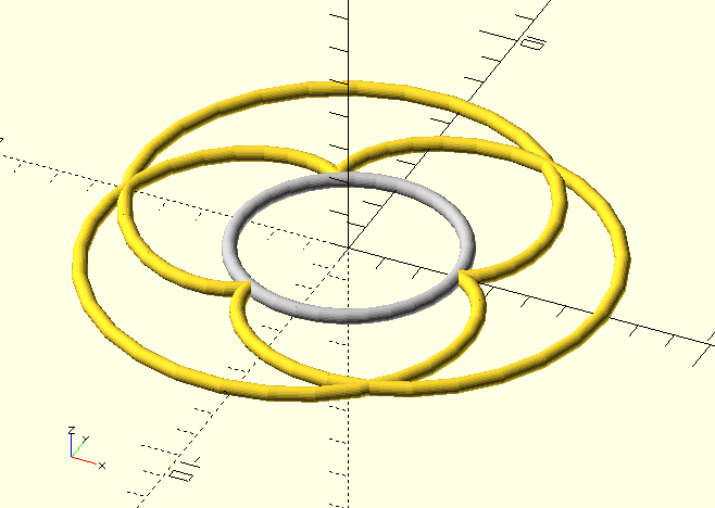
The Circle() module 'draws' a circle; it’s used in images to indicate pitch-circle diameters and such.
|
|
The GHOUL contains a few 'replacement' OpenSCAD routines, one of them is circle(). The reason for this is to get a consistent behaviour among all routines when it comes to circular resolution or 'fragmentation' of circular cross sections.
|
CircleAngles()
CircleAngles(Radius)
-
Radius, scalar, circle radius.
Like ArcAngles() this divides a circle into a set of angles and returns them in a tuple. See below at Segments() for a full explanation of the logic used to calculate the number of divisions.
Segments()
Segments(Radius)
-
Radius, scalar, optional, circle radius.
As a utility function, this really belongs in that section (below), but as it is the 'mother' of all circle-like routines here… Segments() returns the number of segments a circle should be divided into, based on the OpenSCAD special variables, $fa, $fn, and $fs, as well as The GHOUL’s own special variable $ff, which, if not 0, overrides the OpenSCAD special variables and determines the maximum fragment size, as explained in this sidebar:
Nothing is particularly hard if you divide it into small jobs.
The logic Segments() uses to divide a circle is very similar to
OpenSCAD’s own native logic
for dividing circles and arcs into 'fragments' or 'segments', however, The GHOUL is quite particular about having vertices on the cardinal directions, i.e., it requires a four-fold for the vertices of a full circle.
OpenSCAD has three special variables that control how arcs and circles are divided, depending on their respective values and the radius of the arc or circle.
-
$fa the minimum angle for a segment, OpenSCAD default 12, The GHOUL default 6.
-
$fn the number of segments, OpenSCAD default 0, The GHOUL default 0.
-
$fs the minimum size of a segment, OpenSCAD default 2, The GHOUL default 1.
Initially, when determining the number of segments in a circle, The GHOUL first considers these options:
-
If $fn is not 0, it overrides everything, and the segment number will be $fn.
-
If Radius is undefined, we have no dimensional reference, so all we have to go off is angles, and the returned segment number will be 360/$fa, rounded up into a four-fold.
-
If Radius is defined, the segment size will be at least $fs, and the segment number will be no more than 360/$fa, unless $ff is not 0, in which case it overrides $fs and $fa, and the segment size will be no more than $ff, the result of these considerations is then rounded up into a four-fold and returned.
|
|
In case you skipped the sidebar at the beginning; The GHOUL has an additional special variable, $fc, which is used to specify the number of segments of the cross-section of drawn curves such as Arc() and anything drawn by ShowCurve().
|
|
|
If you’re curious how OpenSCAD would have divided a circle, there’s the 'bonus' function Fragments(Radius).
|
 Rant warning…
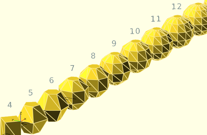
If you think circles in OpenSCAD are a mess, wait till you find out about spheres; the way OpenSCAD constructs those is beyond me. CGI has limits, 3D printers have resolutions, CG spheres are multi-faceted 'balls' that only actually have their true radius at the vertices; all of that’s a given, but…
OpenSCAD uses the same special variables for spheres that it uses to determine the size of circle facets, $fa, $fn, and $fs. But, why the flat poles? why no vertices on the 'equator' half of the time—why is there no equator half the time—and why is it impossible to have a full dimension bounding box, ever—at all? You may accuse me of thinking up a storm in a glass of water, but wouldn’t it be nice if a sphere had a diameter equal to the actual parameter dimension, if not on all three axes, how about in at least one plane?
Arguably, spheres created under an even $fn value have full-radius vertices in the X-Z plane—although not on the X-axis :'( It’s impossible to have full radius vertices on the 'four cardinals', i.e., on the positive and negative X-axis and Y-axis locations. The Z-axis? Let’s not go there; OpenSCAD spheres have flat bloody cropped-off poles…
Spheres have a 'true' equator when they are divided in a multiple of 2 that is not a multiple of 4, this means—of course—that they do not have vertices on the Y-axis, i.e., their Y-dimension is undersize. Their Z-dimension is always undersize. When spheres are divided in a multiple of 4 segments, they’re undersize on all three axes because they don’t have any vertices in the X-Y plane. Spheres divided in an odd number of segments have three different dimensions on the X, Y, and Z axes, and are sliced 'horizontally' in the same manner as a sphere divided into the next even number of segments would be.
Still with me? Convinced that it’s a horror-show yet?
There’s a plethora of ways to generate a sphere,and most are superior to the OpenSCAD method—in my not-so-humble opinion at any rate—I really like the cubesphere; it has full radius vertices in all three orthogonal planes.
There. That hasn’t helped us much, I know, and it makes as good as no difference by the time you’re talking about dimensions that are a significant multiple of your printer’s resolution, especially after your slicer has processed the file, but I thought you should know. And it made me feel better ;-)
Maybe I’ll write my own Sphere() routine one day, with full radius vertices on the three planes, regardless of dimension or special variable settings; it really isn’t rocket science…
Straight lines
ALine()
ALine(Angle,Thickness=0.05,2D=false)
-
Angle, scalar, Line angle CCW from the positive X-axis.
-
Thickness, scalar, line thickness (i.e. width!).
-
Color, OpenSCAD color identifier.
ALine() generates a 'line' through the origin in the Z=0 or X-Y plane, at a given angle to the positive X-axis. Also see HLine(), Line(), and VLine().
All these routines create 'lines'; thin cylinders, unless 2D is true in which case the lines are thin bands of rectangular cross-section, the top surface of which is the Z=0 plane, i.e., they lie beneath the plane. Used by modules such as Dimension() and GraphPaper().
HLine()
HLine(Y,Thickness=0.05,2D=false)
-
Y, scalar, value where the horizontal line crosses the Y-axis.
-
Thickness, scalar, line thickness (i.e. width!).
-
2D, Boolean, draw a '2D' line if true.
HLine() generates a 'line' parallel to the X-axis in the Z=0 or X-Y plane, through a given Y-value. Also see comments at ALine().
Line()
Line(P1,P2,Thickness=0.05,2D=false)
-
P1,P2, points, points between which the line is drawn.
-
Thickness, scalar, line thickness (i.e. width!).
-
Color, OpenSCAD color identifier.
Line() generates a 'line' between two points in the Z=0 or X-Y plane. Also see comments at ALine().
VLine()
VLine(X,Thickness=0.05,2D=false)
-
Y, scalar, value where the vertical line crosses the X-axis.
-
Thickness, scalar, line thickness (i.e. width!).
-
Color, OpenSCAD color identifier.
VLine() generates a 'line' parallel to the Y-axis in the Z=0 or X-Y plane, through a given X-value. Also see comments at ALine().
Utilities
CurveLength()
CurveLength(Array, Closed=false)
-
Array, array, vertices forming a curve.
-
Closed, Boolean, if true the curve is 'closed' and the distance between Array[n] and Array[0] is part thereof.
Returns the developed length of the curve, i.e., the sum of the distances between the successive vertices of the curve.
CurveOffset()
CurveOffset(Curve,Dist,Closed=true)
-
Curve, an array of 2D vertices, describing a curve.
-
Dist, a scalar; offset distance, positive is to the right of Curve when walking Curve beginning-to-end, if Curve is a polygon, this would make the polygon larger.
-
Closed, a Boolean; true if the curve is closed.
CurveOffset() takes a Curve, an array of vertices, and generates a new array, at Dist from Curve. The new array will lie to the right of Curve when 'looking' from the first vertex and Dist is positive.
Curve=[[10, 0],[5,8.7],[-5,8.7],[-10,0],[-5,-8.7],[5,-8.7]]
NewCurve=CurveOffset(Curve,1);
echo(NewCurve);

ECHO: [[11.5, 0], [5.8, 10], [-5.8, 10], [-11.5, 0], [-5.8, -10], [5.8, -10]]
// Note: Values in the above `echo()` output have been rounded to 1 decimal point for purrdyness purposes.
FindCurveVertex()
FindCurveVertex(Curve, Distance, Closed)
-
Curve, array, vertices forming a curve.
-
Distance, distance from the beginning of the curve, i.e., Array[0].
-
Closed, Boolean, Array is a closed curve if true.
Returns the vertex at or before Distance. Takes 'lapping' of a closed curve into account.
TangentPoint()
TangentPoint(Vertex,Curve,Direction=1,Index)
-
Vertex, 2D vertex through (from) which the tangent runs.
-
Curve, vertex array describing a curve.
-
Direction, scalar, if not greater than 0, Curve is searched in reverse direction.
-
Index, integer, vertex from which to start searching. If left undefined, Curve is searched forward from the start if Direction is greater than 0, and backwards from the end if it is not.
Although it doesn’t return a curve, this routine is so closely related to curves that I had a hard time putting it anywhere else (Math and Logic?), so here it is. It searches Curve and returns the first vertex it finds to which the line drawn from Vertex is tangential. Curve can be searched in either direction, from either end, or starting from a certain vertex.
Roulettes
The file TheGHOUL/Lib/Curves/Roulettes.scad contains a number of roulette generating routines, most of which are not really user functions, but deserve attention anyway, because, this is The GHOUL, and nothing is left undocumented. Different kinds of roulettes are used to generate certain parts of tooth-profiles in involute and cycloid gears; also see the documentation at Gears and Clocks.
Roughly speaking, a roulette is the curve described by a point (called the generator or pole) attached to a given curve, as that curve rolls, without slipping, along a second given curve that is fixed.
In the case where the rolling curve is a line, and the generator is a point on the line, the roulette is called an involute of the fixed curve. If the rolling curve is a circle and the fixed curve is a line then the roulette is a trochoid. If, in this case, the point lies on the circle then the roulette is a cycloid.
There is further distinction between epi- and hypo-trochoids (curves outside and inside the fixed circle), and there appear to be several aliases and overlap in the naming—a cycloid is also referred to as a 'common trochoid'—not to mention 'centered trochoids', a moniker that appears to cover a multitude of sins. Then there are the limaçon, cardioid and nephroid, which—really—are all epitrochoids, the deltoid and astroid (which are hypocycloids) are also just (special cases of) hypotrochoids, and, finally (in this by-no-means-complete list), there’s the ellips, created by a circle of radius R rolling inside a circle of radius 2R, with a pole located at r<R. It’s jolly interesting, if you’re into that sort of thing; it made some people a good bit of dosh when they developed the Spirograph at any rate…
Trochoid()
Trochoid(R,r,d,Angle)
-
R, scalar, fixed circle radius.
-
r, scalar, rolling circle radius.
-
d, scalar, generator radius, i.e, the center of the rolling circle to the 'scribing' point.
A trochoid is the curve generated by a point, fixed to a circle which rolls around the inside (hypo-) or outside (epi-) of another, fixed, circle. The point ('pole' or 'generator') can sit on, inside or outside the rolling circle, yielding distinctly different curves. This routine is not here because of the pretty shapes it creates; Epitrochoid and Tusi couple curves are integral to the design of tooth and leaf profiles in clock-gears.
Involute()
Involute(BaseRadius,TipRadius,StartRadius)
-
BaseRadius, scalar, radius of the 'fixed circle'.
-
TipRadius, scalar, radius on which the tooth-tip lies.
-
StartRadius, scalar, radius to start the involute, if not BaseRadius. If left undef, the involute starts on BaseRadius.
You’ll probably not have much use for this routine, but—as you know—this is TheGHOUL, so it must be documented. Here’s a nice image demonstrating how the involute is constructed, and there’s TheGHOUL/DemoFiles/Img_Involute.scad as well, if you’re interested.